Experiment 1
We'll use NumPy and matplotlib for plotting, so import both:
import numpy as np
import matplotlib.pyplot as plt
The data we want to classify comes from two circles, so first define a function to generate some points on a circle (plus some noise):
def circle(radius, sigma=0, num_points=50):
    t = np.linspace(0, 2*np.pi, num_points)
    d = np.zeros((num_points,2), dtype=np.float)
    d[:,0] = radius*np.cos(t) + np.random.randn(t.size)*sigma
    d[:,1] = radius*np.sin(t) + np.random.randn(t.size)*sigma
    return d
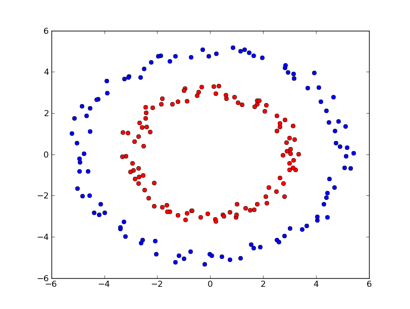
We want to generate 100 training points for each class and 30 points for testing the model, then generate and plot the data:
num_train = 100
num_test = 30
sigma = 0.2

d1 = circle(3, sigma, num_train)
d2 = circle(5, sigma, num_train)

plt.figure()
plt.plot(d1[:,0],d1[:,1],'ro')
plt.plot(d2[:,0],d2[:,1],'bo')
plt.show()
So we get back clearly seperated data:
Now to the SVM. The LibSVM binding expects a list with the classes and a list with the training data:
from svmutil import *

# training data
c_train = []
c_train.extend([0]*num_train)
c_train.extend([1]*num_train)
d_train = np.vstack((circle(3,sigma,num_train), circle(5,sigma,num_train))).tolist()

# test data
c_test = []
c_test.extend([0]*num_test)
c_test.extend([1]*num_test)
d_test = np.vstack((circle(3,sigma,num_test), circle(5,sigma,num_test))).tolist()

problem = svm_problem(c_train,d_train)
The parameters for the model have to be defined (supress output in training):
param = svm_parameter("-q") # quiet!
param.kernel_type=RBF
Our model can now be trained as:
m = svm_train(problem, param)
To get predictions from the model simply pass our test data and the model to svm_predict:
pred_lbl, pred_acc, pred_val = svm_predict(c_test,d_test,m)
and you'll see, the SVM perfectly classifies the data:
>>> p_lbl, p_acc, p_val = svm_predict(c_test,d_test,m)
Accuracy = 100% (60/60) (classification)
But what if the the training data is not that perfect, set sigma to 1:
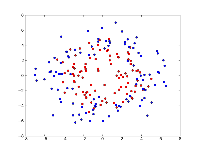
then the default parameters yield:
>>> pred_lbl, pred_acc, pred_val = svm_predict(c_test,d_test,m)
Accuracy = 76.6667% (46/60) (classification)
Often a Grid Search is applied in order to find the best parameters. A Grid Search is nothing but a bruteforce attempt to check all possible parameter combinations. We can easily do that:
results = []
for c in range(-5,10):
  for g in range(-8,4):
    param.C, param.gamma = 2**c, 2**g
    m = svm_train(problem,param)
    p_lbl, p_acc, p_val = svm_predict(c_test,d_test,m)
    results.append([param.C, param.gamma, p_acc[0]])

bestIdx = np.argmax(np.array(results)[:,2])
So the best combination has the parameters:
>>> results[bestIdx]
[0.125, 0.5, 83.333333333333329]
and is with 83.3% only slightly better than default. That's it! The next experiment will use some real life data for prediction.
Experiment 2
The Wine Dataset is a rather simple dataset. It comes as a CSV file and is made up of 178 lines with a class label and 13 properties. In this experiment I want to show you how to use libsvm with Python. Python comes with a built-in csv reader, so it's easy to read in the data:
import csv

reader = csv.reader(open('wine.data', 'rb'), delimiter=',')
classes = []
data = []
for row in reader:
    classes.append(int(row[0]))
    data.append([float(num) for num in row[1:]])
Please note: Always make sure not to include any class labels in your feature vector, because this would make prediction for a SVM trivial and useless.
Now that we have read in the data we'll perform a 10-fold cross validation on the raw data. This will show you that the default RBF and the sigmoid kernel don't work on raw data; both perform only slightly better than random guessing. The linear and polynomial kernel function are better suited for raw data with both having around 95% cross-validation accuracy. I've played with the dataset before and we saw that normalization sometimes matters.
Here is how to do a min-max or z-score normalization with NumPy:
def normalize(X, low=0, high=1, minX=None, maxX=None):
    X = np.asanyarray(X)
    if minX is None:
        minX = np.min(X)
    if maxX is None:
        maxX = np.max(X)
    # Normalize to [0...1].
    X = X - minX
    X = X / (maxX - minX)
    # Scale to [low...high].
    X = X * (high-low)
    X = X + low
    return X

def zscore(X):
    X = np.asanyarray(X)
    return (X-X.mean())/X.std()
On normalized data the RBF performs better with 98% accuracy and the sigmoid kernel has 97%. To finally learn a model you have to switch the cross validation off and train the model on your data. With svm_predict you would generate predictions for your input data. You probably ask yourself now how to normalize unseen input data. If you know the range your inputs can take it is trivial, just do a min-max normalization with the given min and max. If your data is drawn from a stationary process you can assume, that mean and variance doesn't change over time. So you could do a z-score normalization on the new data with the mean and standard deviation from your training data. Note that in the wine example all features were measured on a different scale, so you have to normalize each feature with its mean and standard deviation separately.
Now let's put all this into a script:
from svmutil import *
import numpy as np
import random
import csv

def normalize(X, low=0, high=1):
    X = np.asanyarray(X)
    minX = np.min(X)
    maxX = np.max(X)
    # Normalize to [0...1].
    X = X - minX
    X = X / (maxX - minX)
    # Scale to [low...high].
    X = X * (high-low)
    X = X + low
    return X

def zscore(X):
    X = np.asanyarray(X)
    mean = X.mean()
    std = X.std()
    X = (X-mean)/std
    return X, mean, std

reader = csv.reader(open('wine.data', 'rb'), delimiter=',')
classes = []
data = []
for row in reader:
    classes.append(int(row[0]))
    data.append([float(num) for num in row[1:]])

data = np.asarray(data)
classes = np.asarray(classes)

# normalize data
means = np.zeros((1,data.shape[1]))
stds = np.zeros((1,data.shape[1]))
for i in xrange(data.shape[1]):
    data[:,i],means[:,i],stds[:,i] = zscore(data[:,i])

# shuffle data
idx = np.argsort([random.random() for i in xrange(len(classes))])
classes = classes[idx]
data = data[idx,:]

# turn into python lists again
classes = classes.tolist()
data = data.tolist()

# formulate as libsvm problem
problem = svm_problem(classes, data)

param=svm_parameter("-q")

# 10-fold cross validation
param.cross_validation=1
param.nr_fold=10

# kernel_type : set type of kernel function (default 2)
#   0 -- linear: u'*v
#   1 -- polynomial: (gamma*u'*v + coef0)^degree
#   2 -- radial basis function: exp(-gamma*|u-v|^2)
#   3 -- sigmoid: tanh(gamma*u'*v + coef0)

#param.kernel_type=LINEAR # 95% (raw), 96% (zscore)
#param.kernel_type=POLY # 96% (raw), 97% (zscore)
param.kernel_type=RBF # 43% (raw), 98% (zscore)
#param.kernel_type=SIGMOID # 39% (raw), 98% (zscore)

# perform validation
accuracy = svm_train(problem,param)
print accuracy

# disable cv
param.cross_validation = 0

# training with 80% data
trainIdx = int(0.8*len(classes))
problem = svm_problem(classes[0:trainIdx], data[0:trainIdx])

# build svm_model
model = svm_train(problem,param)

# test with 20% data
# if data was not normalized you would do:
# data = (data-means)/stds
p_lbl, p_acc, p_prob = svm_predict(classes[trainIdx:], data[trainIdx:], model)
print p_acc

# perform simple grid search
#results = []
#for c in range(-3,3):
#   for g in range(-3,3):
#       param.C, param.gamma = 2**c, 2**g
#       acc = svm_train(problem,param)
#       results.append([param.C, param.gamma, acc])

#bestIdx = np.argmax(np.array(results)[:,2])
#print results[bestIdx]