My website recently saw a lot of hits for a tiny wiki page on Local Binary Patterns, so I thought it might be useful to share some code on generating Local Binary Patterns.
All source code in this post is available at:
It comes as a CMake project, so to build and run it simply type:
philipp@mango:~/some/dir$ mkdir build; cd build
philipp@mango:~/some/dir/build$ cmake ..
philipp@mango:~/some/dir/build$ make
philipp@mango:~/some/dir/build$ ./lbp <device id (default 0)>
Python and MATLAB implementations can be obtained from the facerec project at:
If I forgot anything important, I am sure the great Scholarpedia page on Local Binary Patterns answers your questions.
Introduction
If you have read my blog posts on Fisherfaces or Eigenfaces I've left you with the impression everything works just fine. You should have been sceptic.
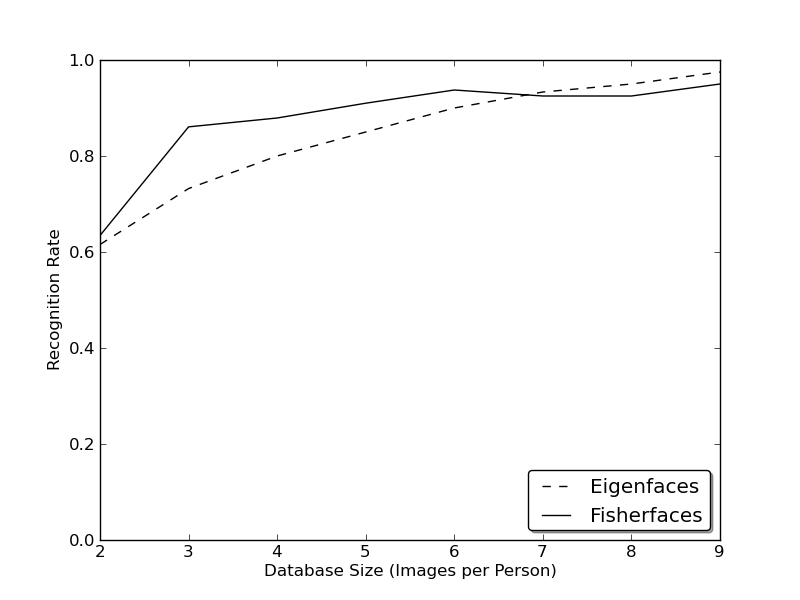
Real life isn't perfect at all. You simply can't guarantee perfect light settings in your images or 10 images of a person. So what if there's only one image for each subject? Our covariance estimates may be wrong, which is something known as the Small Sample Size Problem. Remember the Eigenfaces method had a 96% recognition rate on the AT&T Facedatabase? How many images do we actually need to get such useful estimates?
I've put a tiny script for you into the appendix, feel free to experiment with it. Running the script on the AT&T Facedatabase, which is a fairly easy image database, shows:
So let's have a look at alternative methods for feature extraction.
Local Binary Patterns
The Local Binary Patterns algorithm has its roots in 2D texture analysis. The basic idea is to summarize the local structure in an image by comparing each pixel with its neighborhood.
Take a pixel as center and threshold its neighbors against. If the intensity of the center pixel is greater-equal its neighbor, then denote it with 1 and 0 if not. You'll end up with a
binary number for each pixel, just like 11001111. With 8 surrounding pixels you'll end up with 2^8 possible combinations, which are called Local Binary Patterns or sometimes
abbreviated as LBP codes.
The first LBP operator actually used a fixed 3 x 3 neighborhood just like this:

So why is this description so great? Because it's dead simple to implement and fast as hell. I'll just name it Original LBP in code:
template <typename _Tp>
void lbp::OLBP_(const Mat& src, Mat& dst) {
    dst = Mat::zeros(src.rows-2, src.cols-2, CV_8UC1);
    for(int i=1;i<src.rows-1;i++) {
        for(int j=1;j<src.cols-1;j++) {
            _Tp center = src.at<_Tp>(i,j);
            unsigned char code = 0;
            code |= (src.at<_Tp>(i-1,j-1) > center) << 7;
            code |= (src.at<_Tp>(i-1,j) > center) << 6;
            code |= (src.at<_Tp>(i-1,j+1) > center) << 5;
            code |= (src.at<_Tp>(i,j+1) > center) << 4;
            code |= (src.at<_Tp>(i+1,j+1) > center) << 3;
            code |= (src.at<_Tp>(i+1,j) > center) << 2;
            code |= (src.at<_Tp>(i+1,j-1) > center) << 1;
            code |= (src.at<_Tp>(i,j-1) > center) << 0;
            dst.at<unsigned char>(i-1,j-1) = code;
        }
    }
}
This description enables you to capture very fine grained details in images. In fact the authors were able to compete with state of the art results for texture classification.
Soon after the operator was published it was noted, that a fixed neighborhood fails to encode details differing in scale. So the operator was extended to use a variable neighborhood. The idea is to align an abritrary number of neighbors on a circle with a variable radius, which enables to capture the following neighborhoods:
The operator is an extension to the original LBP codes, so it gets called the Extended LBP (sometimes also referred to as Circular LBP). If a points coordinate on the circle doesn't correspond to image coordinates, the point get's interpolated. Computer science has a bunch of clever interpolation schemes, I'll simply do a bilinear interpolation:
template <typename _Tp>
void lbp::ELBP_(const Mat& src, Mat& dst, int radius, int neighbors) {
    neighbors = max(min(neighbors,31),1); // set bounds...
    // Note: alternatively you can switch to the new OpenCV Mat_
    // type system to define an unsigned int matrix... I am probably
    // mistaken here, but I didn't see an unsigned int representation
    // in OpenCV's classic typesystem...
    dst = Mat::zeros(src.rows-2*radius, src.cols-2*radius, CV_32SC1);
    for(int n=0; n<neighbors; n++) {
        // sample points
        float x = static_cast<float>(radius) * cos(2.0*M_PI*n/static_cast<float>(neighbors));
        float y = static_cast<float>(radius) * -sin(2.0*M_PI*n/static_cast<float>(neighbors));
        // relative indices
        int fx = static_cast<int>(floor(x));
        int fy = static_cast<int>(floor(y));
        int cx = static_cast<int>(ceil(x));
        int cy = static_cast<int>(ceil(y));
        // fractional part
        float ty = y - fy;
        float tx = x - fx;
        // set interpolation weights
        float w1 = (1 - tx) * (1 - ty);
        float w2 =      tx  * (1 - ty);
        float w3 = (1 - tx) *      ty;
        float w4 =      tx  *      ty;
        // iterate through your data
        for(int i=radius; i < src.rows-radius;i++) {
            for(int j=radius;j < src.cols-radius;j++) {
                float t = w1*src.at<_Tp>(i+fy,j+fx) + w2*src.at<_Tp>(i+fy,j+cx) + w3*src.at<_Tp>(i+cy,j+fx) + w4*src.at<_Tp>(i+cy,j+cx);
                // we are dealing with floating point precision, so add some little tolerance
                dst.at<unsigned int>(i-radius,j-radius) += ((t > src.at<_Tp>(i,j)) && (abs(t-src.at<_Tp>(i,j)) > std::numeric_limits<float>::epsilon())) << n;
            }
        }
    }
}
Now using an abritrary radius and sample points has two effects. The more sampling points you take, the more patterns you can encode, the more patterns (and probably information) you have, but the higher the computational effort. Instead the larger the radius, the smoother the LBP image, the larger details can be captured, the less discriminative power the description may have (if you don't increase the sampling points at the same time).
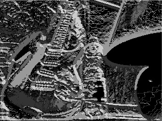
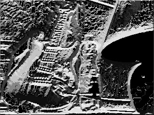
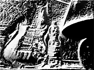
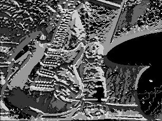
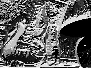
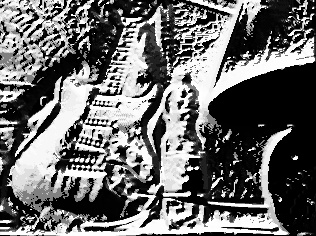
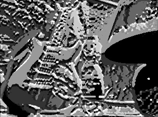
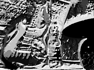
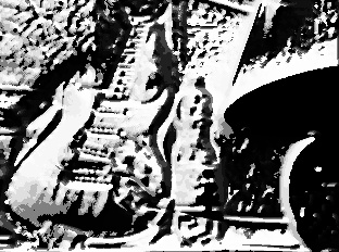
Let's see what the LBP codes look like given a sample frame. My webcam isn't really high-resolution, please don't laugh at my hardware!
Now what's left is how to classify an object.
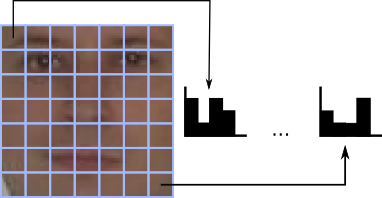
If you would throw all features into a single histogram all spatial information is discarded. In tasks like face detection (and a lot of other pattern recognition problems) spatial information is very useful, so it has to be incorporated into the histogram somehow. The representation proposed by Ahonen et al. in Face Recognition with Local Binary Patterns is to divide the LBP image into grids and build a histogram of each cell seperately.
Then by concatenating the histograms the spatial information is encoded (not merging them), just like this:
This informal description translates to OpenCV as:
And here's the Local Binary Patterns Histograms Face Recognizer:
Notes
The experiment was done with facerec version number 0.1. If you want to recreate them you either download the tag or you adapt the script to the most recent version (which should be very easy).
