Introduction
Some time ago I have written a post on Linear Discriminant Analysis, a statistical method often used for dimensionality reduction and classification. It was invented by the great statistician Sir R. A. Fisher, who successfully used it for classifying flowers in his 1936 paper "The use of multiple measurements in taxonomic problems" (The famous Iris Data Set is still available at the UCI Machine Learning Repository.). But why do we need another dimensionality reduction method, if the Principal Component Analysis (PCA) did such a good job? Well, the PCA finds a linear combination of features that maximizes the total variance in data. While this is clearly a powerful way to represent data, it doesn't consider any classes and so a lot of discriminative information may be lost when throwing some components away. This can yield bad results, especially when it comes to classification. In order to find a combination of features that separates best between classes the Linear Discriminant Analysis instead maximizes the ration of between-classes to within-classes scatter. The idea is that same classes should cluster tightly together.
This was also recognized by Belhumeur, Hespanha and Kriegman and so they applied a Discriminant Analysis to face recognition in their paper "Eigenfaces vs. Fisherfaces: Recognition Using Class Specific Linear Projection" (1997). The Eigenfaces approach by Pentland and Turk as described in "Eigenface for Recognition" (1991) was a revolutionary one, but the original paper already discusses the negative effects of ima ges with changesn background, light and perspective. So on datasets with differences in the setup, the Principal Component Analysis is likely to find the wrong components for classification and can perform poorly.
You seldomly see something explained with code and examples, so I thought I'll change that. And there are already so many libraries, why not add another one? I have prepared a Python and GNU Octave/MATLAB version. The code is available in my github repository at:
I've put all the code under a BSD License, so feel free to use it for your projects. While this post is based on the very first version number 0.1 of the framework, it still outlines the concepts in detail. You won't have any troubles to reproduce the results with the latest sources, I've added a comprehensive README to the project.
There's also a much simpler implementation in the documents over at:
- https://bytefish.de/pdf/facerec_python.pdf (Python version)
- https://bytefish.de/pdf/facerec_octave.pdf (GNU Octave/MATLAB version)
You'll find all code shown in these documents in the projects github repository:
Algorithmic Description
The Fisherfaces algorithm we are going to implement basically goes like this:
- Construct the Imagematrix
Xwith each column representing an image. Each image is a assigned to a class in the corresponding class vectorC. - Project
Xinto the(N-c)-dimensional subspace asPwith the rotation matrixWPcaidentified by a Principal Component Analysis, whereNis the number of samples inXcis unique number of classes (length(unique(C)))
- Calculate the between-classes scatter of the projection
PasSb = \sum_{i=1}^{c} N_i*(mean_i - mean)*(mean_i - mean)^T, wheremeanis the total mean ofPmean_iis the mean of classiinPN_iis the number of samples for classi
- Calculate the within-classes scatter of
PasSw = \sum_{i=1}^{c} \sum_{x_k \in X_i} (x_k - mean_i) * (x_k - mean_i)^T, whereX_iare the samples of classix_kis a sample ofX_imean_iis the mean of classiinP
- Apply a standard Linear Discriminant Analysis and maximize the ratio of the determinant of between-class scatter and within-class scatter. The solution is given by the set of generalized eigenvectors
WfldofSbandSwcorresponding to their eigenvalue. The rank ofSbis atmost(c-1), so there are only(c-1)non-zero eigenvalues, cut off the rest. - Finally obtain the Fisherfaces by
W = WPca * Wfld.
For a detailed description of the algorithms used in this post, please refer to the paper in Further Reading.
Implementation Details
Enough talk, show me the code! I will focus on the Python version, because it's a lot cleaner. Don't get me wrong, most of the functions are also implemented in GNU Octave and it's also easy to use. Aside from architectural aspects, translating the core algorithms from Octave to Python was almost trivial. Thanks again to NumPy and matplotlib, which make Python feel like GNU Octave/MATLAB. This is great due to the fact, that OpenCV uses NumPy arrays since OpenCV2.2. That makes it possible to integrate NumPy projects into an OpenCV project without any hassle -- rapid prototyping comes for free!
Since the Fisherfaces method performs a Principal Component Analysis and Linear Discriminant Analysis on the data, all we need are two classes to perform a PCA and LDA. The Fisherfaces method then essentially boils down to (comments stripped off):
class Fisherfaces(Model):

    def __init__(self, X=None, y=None, num_components=None, k=1):
        Model.__init__(self, name="Fisherfaces")
        self.k = k
        self.num_components = num_components
        try:
            self.compute(X,y)
        except:
            pass


    def compute(self, X, y):
        """ Compute the Fisherfaces as described in [BHK1997]: Wpcafld = Wpca * Wfld.

        Args:
            X [dim x num_data] input data
            y [1 x num_data] classes
        """
        n = len(y)
        c = len(np.unique(y))
        pca = PCA(X, n-c)
        lda = LDA(pca.project(X), y, self.num_components)
        self._eigenvectors = pca.W*lda.W
        self.num_components = lda.num_components
        self.P = self.project(X)
        self.y = y

    def predict(self, X):
        Q = self.project(X)
        return NearestNeighbor.predict(self.P, Q, self.y, k=self.k)

    def project(self, X):
        return np.dot(self._eigenvectors.T, X)

    def reconstruct(self, X):
        return np.dot(self._eigenvectors, X)
All models in the code derive from a generic Model((Which does absolutely nothing, I just thought it would make a nice OOP hierarchy...)) and implement a compute and predict method, which are used to estimate the performance of a classifier with a cross validation. Classes for performing a leave-one-out and k-fold cross validation are implemented. I only measure the recognition rate of a classifier, so something for your use case might be missing. Feel free to add your measures in the validation module.
The filereader module only has a FilesystemReader right now. It loads images in a given path, assuming a folder structure of <path>/<subject>/<image> for reading in the dataset. There are some limitations, which will be fixed in later versions. For now you must ensure, that all images have equal size and the image format is supported by PIL (same applies for ImageMagick in GNU Octave).
Last but not least, there's a visualization module. I don't feel afraid to say: it feels very, very hardcoded. Plotting and subplotting eigenvectors is supported, so is comparing accuracy (+ standard deviation) vs. parameters for a bunch of validators (errorbar plot). Absolutely everything regarding the style of a plot is missing, so it will take a lot more iterations to create smoother plotting facilities. If you want to quickly create some plots, go for the Octave version for now.
Experiments
Everything is implemented? So let the experiments begin! The last face recognition experiment I have posted was performed on the AT&T Face database. Now if you spider through some literature you will notice, that it's a rather easy dataset. Images are taken in a very controlled environment with only slightly changes in perspective and light. You won't see any great improvements with a Discriminant Analysis, because it's hard to beat the 96% accuracy we got with Eigenfaces.
That's why I will validate the algorithms on the Yale Facedatabase A. You can download it from the UCSD Computer Vision Group:
The second experiment is something I wanted to do for a long time: we will see how faces of celebrities cluster together and I can finally project my face to where it belongs (hopefully I belong to the Brad Pitt cluster)! You'll see dramatic improvements with a Linear Discriminant Analysis in this experiment.
Validation scheme
My experimental validation scheme is very easy. I will do n runs for each experiment and each run is validated with a k-fold Cross-validation on a shuffled training set. From these n runs the average accuracy and standard deviation is reported. In literature you'll often find the results of a Leave-One-Out Cross Validation, so I'll also report it. For a good writeup on cross validation based model selection, see Andrew Moore's slides on Cross-validation for preventing and detecting overfitting.
k-fold Cross Validation
Cross-... what? Imagine I want to estimate the error of my face recognition algorithm. I have captured images of people over a long period of time and now I am building a training and test set from these images. Somehow I have managed to put all happy looking people in the training set, while all people in my test set are terribly sad with their head hanging down somewhere. Should I trust the results I get from this evaluation? Probably not, because it's a really, really unfortunate split of my available data. A cross-validation avoids such splits, because you build k (non-overlapping) training and test datasets from your (shuffled) original dataset. So what's a fold then? It's best explained with an example.
For a dataset D with 3 classes {c0,c1,c2} each having 4 observations {o0,o1,o2,o3}, a 4-fold cross validation produces the following four folds F:
(F1)

    o0 o1 o2 o3
c0 | A  B  B  B |
c1 | A  B  B  B |
c2 | A  B  B  B |

A = {D[c0][o0], D[c1][o0], D[c2][o0]}
B = D\A

(F2)

    o0 o1 o2 o3
c0 | B  A  B  B |
c1 | B  A  B  B |
c2 | B  A  B  B |

A = {D[c0][o1], D[c1][o1], D[c2][o1]}
B = D\A

(F3)

    o0 o1 o2 o3
c0 | B  B  A  B |
c1 | B  B  A  B |
c2 | B  B  A  B |

A = {D[c0][o2], D[c1][o2], D[c2][o2]}
B = D\A

(F4)

    o0 o1 o2 o3
c0 | B  B  B  A |
c1 | B  B  B  A |
c2 | B  B  B  A |

A = {D[c0][o3], D[c1][o3], D[c2][o3]}
B = D\A
From these folds the accuracy and the standard deviation can be calculated. Please have a look at the Python or GNU Octave implementations if you have troubles implementing it. It's pretty self-explaining.
Leave One Out Cross Validation
A Leave-one-out cross-validation (LOOCV) is the degenerate case of a k-fold cross-validation, where k is chosen to be the number of observations in the dataset. Simply put, you use one observation for testing your model and the remaining data for training the model. This results in as many experiments as observations available, which may be too expensive for large datasets.
For the same example as above you would end up with the following 12 folds F in a LOOCV:
(F1)

    o0 o1 o2 o3
c0 | A  B  B  B |
c1 | B  B  B  B |
c2 | B  B  B  B |

A = {D[c0][o0]}
B = D\A

(F2)

    o0 o1 o2 o3
c0 | B  A  B  B |
c1 | B  B  B  B |
c2 | B  B  B  B |

A = {D[c0][o1]}
B = D\A

(...)

(F12)
    o0 o1 o2 o3
c0 | B  B  B  B |
c1 | B  B  B  B |
c2 | B  B  B  A |

A = {D[c2][o3]}
B = D\A
Yale Facedatabase A
The first database I will evaluate is the Yale Facedatabase A. It consists of 15 people (14 male, 1 female) each with 11 grayscale images sized 320x243px. There are changes in the light conditions (center light, left light, right light), background and in facial expressions (happy, normal, sad, sleepy, surprised, wink) and glasses (glasses, no-glasses).
Data Preprocessing
Unfortunately the images in this database are not aligned, so the faces may be at different positions in the image. For the Eigenfaces and Fisherfaces method the images need to be preprocessed, since both methods are sensible to rotation and scale. You don't want to do this manually, so I have written a function crop.m/crop_face.py for this, which has the following description:
function crop(filename, eye0, eye1, top, left, dsize)
    %% Rotates an image around the eyes, resizes to destination size.
    %%
    %% Assumes a filename is structured as ".../subject/image.extension", so that
    %% images are saved in a the folder (relative to where you call the script):
    %%  "crop_<subject>/crop_<filename>"
    %%
    %% Args:
    %%  filename: Image to preprocess.
    %%  eye0: [x,y] position of the left eye
    %%  eye1: [x,y] position of the right eye
    %%  top: percentage of offset above the eyes
    %%  left: percentage of horizontal offset
    %%  dsize: [width, height] of destination filesize
    %%
    %% Example:
    %% crop("/path/to/file", [300, 100], [380, 110], 0.3, 0.2, [70,70])
    %%
    %% Leaves 21px offset above the eyes (0.3*70px) and 28px horizontal
    %% offset. 20% of the image to the left eye, 20% to the right eye
    %% (2*0.2*70=28px).
I specify the dimensions of the cropped image to be (100,130) for this database. top is the vertical offset, which specifies how much of the image is above the eyes, 40% seems to be a good value for these images. left specifies the horizontal offset, how much space is left from an eye to the border, 30% is a good value. The image is then rotated by the eye positions. If it's not desired to align all images at the eyes, scale or rotate them, please adjust the script to your needs. batch_crop.m is a simple script to crop images given by their filename and associated eye coordinates. Feel free to translate it to Python.
After having preprocessed the images (coordinates for this database are given here) you'll end up with subsets for each person like this (function used to create the gallery of images):

The preprocessed dataset then has to be stored in a hierarchy similiar to this:
philipp@mango:~/python/facerec$ tree /home/philipp/facerec/data/yalefaces
/home/philipp/facerec/data/yalefaces
|-- s01
|   |-- crop_subject01.centerlight
|   |-- crop_subject01.glasses
|   |-- crop_subject01.happy
|       [...]
|-- s02
|   |-- crop_subject02.centerlight
|   |-- crop_subject02.glasses
|   |-- crop_subject02.happy
|       [...]

15 directories, 165 files
Eigenfaces
I want to do face recognition on this dataset. The Eigenfaces method did such a good job on the AT&T Facedatabase, so how does it work for the Yalefaces? Let's find out and import the models, validation and filereader:
>>> from facerec.models import *
>>> from facerec.validation import *
>>> from facerec.filereader import *
Read in the Yale Facedatabase A:
>>> dataset = FilesystemReader("/home/philipp/facerec/data/yalefaces")
Create the Eigenfaces model, we'll take the 50 principal components in this example:
>>> eigenface = Eigenfaces(num_components=50) # take 50 principal components
We can measure the performance of this classifier with a Leave-One Out Cross validation:
>>> cv0 = LeaveOneOutCrossValidation(eigenface)
>>> cv0.validate(dataset.data,dataset.classes,print_debug=True)
>>> cv0
Leave-One-Out Cross Validation (model=Eigenfaces, runs=1, accuracy=81.82%, tp=135, fp=30, tn=0, fn=0)
So the model has a recognition rate of 81.82%. Note that a Leave-One-Out Cross validation can be computationally expensive for large datasets. In this example we are computing 165 models, with a computation time of 3 seconds per model this validation will take circa 8 minutes to finish. It's often more useful to perform a k-fold cross validation instead, because a Leave One Out Cross validation can also act weird at times (see the slides at Introduction to Pattern Analysis: Cross Validation). A 5-fold cross validation is good for this database:
>>> cv1= KFoldCrossValidation(eigenfaces, k=5) # perform a 5-fold cv
>>> for i in xrange(10):
...     cv1.validate(dataset.data,dataset.classes, print_debug=True)
The model will be validated 50 times in total, so the loop will take 2.5 minutes to finish. If you want to log the validation results per fold (so you can get the standard deviation of a single k-fold cross-validation run for example) add results_per_fold=True when initializing the class (be careful, the figures may be misleading for very small folds).
Some coffees later the validation has finished. Before reporting the final figure I'd like to show you some methods common to all validation objects:
>>> cv1.results
array([[123,  27,   0,   0],
       [123,  27,   0,   0],
       [121,  29,   0,   0],
       [119,  31,   0,   0],
       [120,  30,   0,   0],
       [121,  29,   0,   0],
       [122,  28,   0,   0],
       [124,  26,   0,   0],
       [120,  30,   0,   0],
       [121,  29,   0,   0]])
>>> cv1.tp
array([123, 123, 121, 119, 120, 121, 122, 124, 120, 121])
>>> cv1.accuracy
0.80933333333333335
>>> cv1.std_accuracy
0.0099777436361914683
And to get an overview you can simply get the representation of the Validation object:
>>> cv1 # or simply get the representation
k-Fold Cross Validation (model=Eigenfaces, k=5, runs=10, accuracy=80.93%, std(accuracy)=1.00%, tp=1214, fp=286, tn=0, fn=0)
With 80.93%+-1.00% accuracy the Eigenfaces algorithms performs OK on this dataset, I wouldn't say it performs bad. But can we do better, by taking less or more principal components? We can write a small script to evaluate that. I will perform a 5-fold cross-validation on the Eigenfaces model with [10, 25, 40, 55, 70, 85, 100] components:
parameter = range(10,101,15)
results = []
for i in parameter:
    cv = KFoldCrossValidation(Eigenfaces(num_components=i),k=5)
    cv.validate(dataset.data,dataset.classes)
    results.append(cv)
And we can see, that it doesn't really better the recognition rate:
>>> for result in results:
...     print "%d components: %.2f%%+-%.2f%%" % (result.model.num_components, result.accuracy*100, result.std_accuracy*100)
...
10 components: 73.33%+-0.00%
25 components: 80.00%+-0.00%
40 components: 80.67%+-0.00%
55 components: 81.33%+-0.00%
70 components: 82.67%+-0.00%
85 components: 81.33%+-0.00%
100 components: 82.00%+-0.00%
Maybe we can get a better understanding of the method if we look at the Eigenfaces. Computing the model is necessary, because in the validation the model is cleared.
>>> eigenfaces = Eigenfaces(dataset.data,dataset.classes,num_components=100) # model will now be computed
and then plot the Eigenfaces:
>>> from facerec.visual import *
>>> PlotSubspace.plot_weight(model=eigenfaces, num_components=16, dataset=dataset, title="Eigenfaces", rows=4, cols=4, filename="16_eigenfaces.png")
Almost everywhere you see grayscaled Eigenfaces, which are really hard to explain. With a colored heatmap instead you can easily see the distribution of grayscale intensities, where 0 codes a dark blue and 255 is a dark red:

Just by looking at the first 16 Eigenfaces we can see, that they don't really describe facial features to distinguish between persons, but find components to reconstruct from. The fourth Eigenface for example describes the left-light, while the principal component 6 describes the right-light. This makes sense if you think of the Principal Component Analysis not as a classification method, but more as a compression method.
Let's see what I mean. By computing the Eigenfaces, we have projected the database onto the first hundred components as identified by a Principal Component Analysis. This effectively reduced the dimensionality of the images to 100. We can now try to reconstruct the real faces from these 100 components:
>>> proj1 = eigenfaces.P[:,17].copy()
>>> I = eigenfaces.reconstruct(proj1)
... and plot it:
>>> PlotBasic.plot_grayscale(I, "eigenface_reconstructed_face.png", (dataset.width, dataset.height))
... and we should see a face again:

Fisherfaces
Time for the Fisherfaces method! If you haven't done already, import the modules and load the data:
>>> from facerec.models import *
>>> from facerec.validation import *
>>> from facerec.filereader import *
Read the dataset:
>>> dataset = FilesystemReader("/home/philipp/facerec/data/yalefaces")
create the model (default parameters are ok):
>>> fisherfaces = Fisherfaces()
And then perform a Leave-One-Out Cross-Validation:
>>> cv2 = LeaveOneOutCrossValidation(fisherfaces)
>>> cv2.validate(dataset.data,dataset.classes, print_debug=True)
>>> cv2
Leave-One-Out Cross Validation (runs=1, accuracy=96.36%, tp=159, fp=6, tn=0, fn=0)
... which yields an accuracy of 96.36%. Performing 10 runs of a 5-fold cross validation supports this:
>>> cv3 = KFoldCrossValidation(fisherfaces, k=5) # perform a 5-fold cv
>>> for i in xrange(10):
...     cv3.validate(X,y,print_debug=True)
>>> cv3
k-Fold Cross Validation (k=5, runs=10, accuracy=96.80%, std(accuracy)=1.63%, tp=1452, fp=48, tn=0, fn=0, model=Fisherfaces (num_components=14))
Allthough the standard deviation is slightly higher for the Fisherfaces, with 96.80%+-1.63% it performs much better than the Eigenfaces method. You can also see that the faces were reduced to only 14 components (equals number of subjects - 1). Let's have a look at the components identified by the Fisherfaces method:
>>> fisherface = Fisherfaces(dataset.data,dataset.classes) # initialize and compute, or call compute explicitly
Import the visual module and plot the faces:
>>> from facerec.visual import *
>>> PlotSubspace.plot_weight(model=fisherface, num_components=14, dataset=dataset, filename="16_fisherfaces.png", rows=4, cols=4)
The Fisherfaces are a bit harder to explain, because they identify regions of a face that separate faces best from each other. None of them seems to encode particular light settings, at least it's not as obvious as in the Eigenfaces method:
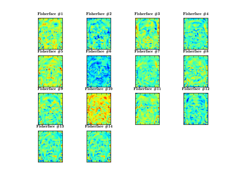
I could only guess which component describes which features. So I leave the interpretation up to the reader. What we lose with the Fisherfaces method for sure, is the ability to reconstruct faces. If I want to reconstruct face number 17, just like in the Eigenfaces section:
>>> proj2 = fisherface.P[:,17].copy()
>>> I2 = fisherface.reconstruct(proj2)
... and plot it:
>>> PlotBasic.plot_grayscale(I2, "fisherface_reconstructed_face.png", (dataset.width, dataset.height))
We get back a picture similar to:

Conclusion
On this dataset the Fisherface method performed much better, than the Eigenfaces method did. While it yields a much better recognition performance, the ability to reconstruct faces from the Eigenspace is lost. So in conclusion, I think both methods complement each other. It would be a good idea to keep the PCA object around (already computed in the Fisherfaces method) in order to use its reconstruction capabilities.
Celebrities Dataset
Some years ago a lot of people told me, that I am looking just like Brad Pitt. Or did I tell it everyone after seeing Troy for the fifth time? Whatever -- sadly times have changed. I am losing my hair and now I am exponentially progressing towards a Sir Patrick Stewart or a bald Britney Spears. Now armed with the algorithms we've discussed, I can finally clear the confusion and find out which celebrity I resemble the most! This last experiment turned into a weekend project itself, but I had a lot of fun writing it and I hope you have fun reading it.
My celebrity dataset consists of the following faces:
- Angelina Jolie
- Arnold Schwarzenegger
- Brad Pitt
- George Clooney
- Johnny Depp
- Justin Timberlake
- Katy Perry
- Keanu Reeves
- Patrick Stewart
- Tom Cruise
I have chosen the images to be frontal face with a similiar perspective and light settings. Since the algorithms are sensible towards rotation and scale, the images have been preprocessed to equal scale of 70x70px and centered eyes. Here is my Clooney-Set for example:

I hope you understand that I can't share the dataset with you. Some of the photos have a public license, but most of the photos have an unclear license. From my experience all I can tell you is: finding images of George Clooney took less than a minute, but it was really, really hard finding good images of Johnny Depp or Arnold Schwarzenegger.
Recognition
Let's see how both methods perform on the celebrities dataset.
Import the modules:
>>> from facerec.models import *
>>> from facerec.validation import *
>>> from facerec.filereader import *
>>> from facerec.visual import *
Read in the database:
>>> dataset = FilesystemReader("/home/philipp/facerec/data/c1")
The Eigenfaces method with a Leave-One-Out cross validation:
>>> eigenface = Eigenfaces(num_components=100)
>>> cv0 = LeaveOneOutCrossValidation(eigenface)
>>> cv0.validate(dataset.data,dataset.classes,print_debug=True)
>>> cv0
Leave-One-Out Cross Validation (model=Eigenfaces, runs=1, accuracy=44.00%, tp=44,
 fp=56, tn=0, fn=0)
Only achieves 44% recognition rate! A 5-fold cross validation:
>>> cv1 = KFoldCrossValidation(eigenface, k=5)
>>> for i in xrange(10):
...     cv1.validate(dataset.data,dataset.classes,print_debug=True)
>>> cv1
k-Fold Cross Validation (model=Eigenfaces, k=5, runs=10, accuracy=43.30%,
 std(accuracy)=2.33%, tp=433, fp=567, tn=0, fn=0)
Shows that the recognition rate of 43.30%+-2.33% is a bit better than guessing, still it's too bad to decide between celebrities.
The Fisherface method instead:
>>> fisherface = Fisherfaces()
... achieves a 93% recognition rate with a leave one out strategy:
>>> cv2 = LeaveOneOutCrossValidation(fisherface)
>>> cv2.validate(dataset.data,dataset.classes, print_debug=True)
Leave-One-Out Cross Validation (model=Fisherfaces, runs=1, accuracy=93.00%, tp=93,
 fp=7, tn=0, fn=0)
And with 5-fold cross validation:
>>> cv3 = KFoldCrossValidation(fisherface,k=5)
>>> for i in xrange(10):
...     cv3.validate(dataset.data,dataset.classes,print_debug=True)
>>> cv3
k-Fold Cross Validation (model=Fisherfaces (num_components=9), k=5, runs=10,
accuracy=90.50%, std(accuracy)=1.36%, tp=905, fp=95, tn=0, fn=0)
... it has a recognition rate of 90.50%+-1.36%. So it's a good classificator to decide between our celebrities. Now let's have a look at the components found by both methods!
Compute both models (necessary because the validation empties the model):
>>> eigenface = Eigenfaces(dataset.data,dataset.classes,num_components=100)
>>> fisherface = Fisherfaces(dataset.data,dataset.classes)
The Eigenfaces...
>>> PlotSubspace.plot_weight(model=eigenface, num_components=16, dataset=dataset, title="Celebrity Eigenface", rows=4, cols=4, filename="16_celebrity_eigenfaces.png")
... again encode light in the images, see the second Eigenface for example:

While the Fisherfaces identify regions:
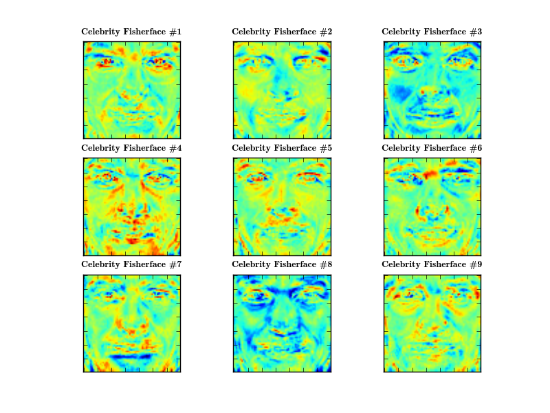
>>> PlotSubspace.plot_weight(model=fisherface, num_components=9, dataset=dataset, title="Celebrity Fisherface", rows=3, cols=3, filename="9_celebrity_fisherfaces.png")
... where you can decide between the persons. The first component for example describes the eyes, while other components describe mouth-ness or eye-browness of a face:
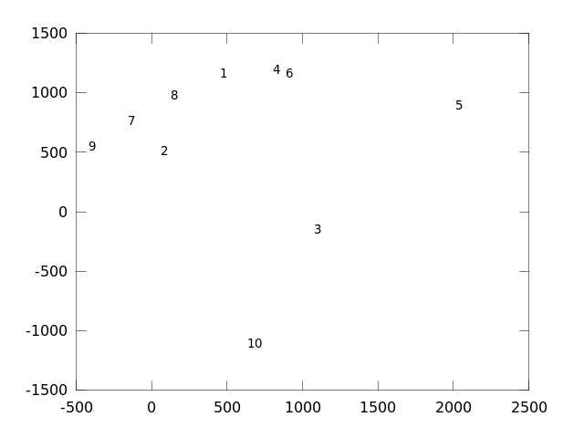
By using two and three components, we can see how the faces are distributed (using GNU Octave, see fisherfaces_example.m). I'll use just one example per class for a better overview:
octave:1> addpath (genpath ("."));
octave:2> [X y width height names] = read_images("/home/philipp/facerec/data/c1");
octave:3> fisherface = fisherfaces(X,y);
octave:4> figure; hold on
octave:5> for i = [1:10]
> C = findclasses(fisherface.y, i)
> text(fisherface.P(1,C(1)), fisherface.P(2,C(1)), num2str(i));
> endfor
octave:6> print -dpng "-S640,480" celebrity_facespace.png
octave:7> names
names =

{
  [1,1] = crop_angelina_jolie
  [1,2] = crop_arnold_schwarzenegger
  [1,3] = crop_brad_pitt
  [1,4] = crop_george_clooney
  [1,5] = crop_johnny_depp
  [1,6] = crop_justin_timberlake
  [1,7] = crop_katy_perry
  [1,8] = crop_keanu_reeves
  [1,9] = crop_patrick_stewart
  [1,10] = crop_tom_cruise
}
Brad Pitt (3), Johnny Depp (5) and Tom Cruise (10) seem to have a unique face, as they are far away from all other faces. Surprisingly George Clooney (4) and Justin Timberlake (6) are near to each other. Arnold Schwarzenegger (2), Katy Perry (7), Keanu Reeves (8) and Patrick Stewart (9) are also close to each other. Angelina Jolie (1) is right between those two clusters; with George Clooney (4) and Keanu Reeves (8) as closest match:
Who Am I?
Now let's finally answer the question why I wrote this post at all. Who do I resemble the most? I'll use a frontal photo of myself and crop it, just like I did with the other faces:

Then I compute the model:
>>> fisherface = Fisherfaces(dataset.data,dataset.classes)
Read in my face:
>>> Q = FilesystemReader.read_image("/home/philipp/crop_me.png")
And find the closest match:
>>> prediction = fisherface.predict(Q)
>>> print dataset.className(prediction)
...
crop_patrick_stewart
I knew it. The closest match to my face is Patrick Stewart. Taking the 5 nearest neighbors, doesn't change a thing... it's still Patrick. Damn, I knew including him would change everything -- and I am not even close to Brad Pitt!
If I project my face on the first 2 components I would actually resemble Arnie the most:

But including the third dimension (projection on second and third component) brings me closer to Patrick Stewart:

Just because the Eigenfaces algorithm can't classify the persons doesn't mean we can't use it here aswell. It did a great job at reconstructing a projected vector, so if I project my face into the facespace... and reconstruct it... my face should be the mixture of those faces.
Let's see what I look like:
>>> eigenface = Eigenfaces(num_components=100)
>>> eigenface.compute(dataset.data,dataset.classes)
>>> proj = eigenface.project(Q)
>>> rec = eigenface.reconstruct(proj)
>>> PlotBasic.greyscale(rec, "philipp_celebrity.png")
Sorry it's a bit small, because my training images are only 70x70 pixels:
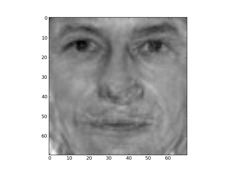
Definitely some Schwarzenegger in there!
Working with the GNU Octave version
The GNU Octave version is just as simple to use as the Python version. I think there's no need to explain every function argument in detail, the code is short and it's all commented in the definition files already. Let's go and fire up Octave. But before you start to do anything, you have to add the path of definition files to the GNU Octave search path. Since GNU Octave 3 you can use addpath(genpath("/path/to/folder/")) to add all definition files in a folder and subfolder:
addpath (genpath ("."));
This makes all function definition in the subfolders available to GNU Octave (see the examples in facerec) and now you can read in the dataset:
% load data
[X y width height names] = read_images("/home/philipp/facerec/data/yalefaces_recognition");
from this we can learn the Eigenfaces with 100 principal components:
eigenface = eigenfaces(X,y,100);
If we want to see the classes in 2D:
%% 2D plot of projection (add the classes you want)
figure; hold on;
for i = findclasses(eigenface.y, [1,2,3])
    text(eigenface.P(1,i), eigenface.P(2,i), num2str(eigenface.y(i)));
endfor
I adopted the KISS principle for the validation. The key idea is the following: the validation gets two function handles fun_train, which learns a model and fun_predict, which tests the learned model. Inside the validation a data array and corresponding classes are passed to the training function; and fun_predict gets a model and test instance. What to do if you need to add parameters to one of the calls? Bind them! I want to learn eigenfaces with 100 components and the prediction should use a 1 nearest neighbor for the classification:
fun_eigenface = @(X,y) eigenfaces(X,y,100);
fun_predict = @(model, Xtest) eigenfaces_predict(model, Xtest, 1)
Easy huh? Performing validations can now be done with:
% perform a Leave-One-Out Cross Validation
cv0 = LeaveOneOutCV(X,y,fun_eigenface, fun_predict, 1)
% perform a 10-fold cross validation
cv1 = KFoldCV(X,y,10,fun_eigenface, fun_predict,1)
% perform a 3-fold cross validation
cv2 = KFoldCV(X,y,3,fun_eigenface, fun_predict,1)
From these results you can gather the same statistics I have used in the Python version. I hope you acknowledge that this version is just as easy to use as the Python version. There are some additional parameters for the functions, so please read the function definition files or the examples to understand those. For further questions, simply comment below.
Conclusion and Lessons learned
In this post I have presented you a simple framework to evaluate your face recognition algorithms with Python and GNU Octave. The Python version will see some updates in the future and its usage might change a little, because some things are too complicated right now. I don't know if maintaining the GNU Octave version pays off, because I'd like to use it for prototyping algorithms. And after all, you have been answered one of most important questions in universe: my face resembles Patrick Stewart.
There are a few lessons I've learnt in this project and I'd like to share. If you are working with large datasets like with hundreds of face images, be sure to always choose the appropriate type for your data: a grayscale image for example only takes values in a range of [0,255] and fits into an unsigned byte. It would be a horrible waste of memory to take floats, which is the default NumPy datatype for arrays and matrices. And this applies to every other dataset as well. If you know which values your inputs can take: choose the appropriate type.
Working with NumPy arrays
One thing you have to get used to when starting with NumPy is working with its arrays and matrices. In NumPy it's a rule of thumb to take NumPy arrays for everything, so if you use one of NumPys built-in functions you can be pretty sure that an array is returned. And there are certain differences to a NumPy matrix you should know about. I've run into the following problem: I wanted to subtract the column mean from each column vector of an array A. My first version was like this:
>>> A = np.array([[2,2],[2,7]])
>>> A - A.mean(axis=1)
array([[ 0. , -2.5],
       [ 0. ,  2.5]])
>>> A.mean(axis=1)
array([ 2. ,  4.5])
Which is obvliously wrong and it is because A.mean(axis=1) returns a row instead of a column, as you can see in the listing. You can avoid that with:
>>> A - A.mean(axis=1).reshape(-1,1)
array([[ 0. ,  0. ],
       [-2.5,  2.5]])
>>> # or you set the metadata information to a matrix
>>> A = np.asmatrix(A)
>>> A - A.mean(axis=1)
matrix([[ 0. ,  0. ],
        [-2.5,  2.5]])
So if you want to treat an array like a matrix, then simply call numpy.asmatrix at some point in your code. Next thing you'll need to understand is related to array slicing and indexing, which is a great thing in NumPy. If you want to just slice the first column off an array, be sure to always make a copy of the sliced data instead of just assigning a variable to the slice. This applies if you don't go for speed, the situation might change if you are looping through data a million times. See this little example. Let's start the interactive python shell and import numpy:
>>> import numpy as np
With pmap we can now see how much memory the python process currently consumes:
philipp@mango:~$ ps ax | grep python
27241 pts/7    S+     0:00 python
philipp@mango:~$ pmap -x 27241
[...]
b783c000       0     524     524 rw---    [ anon ]
b78d7000       0       8       8 rw---    [ anon ]
bf979000       0     172     172 rw---    [ stack ]
-------- ------- ------- ------- -------
total kB   26436       -       -       -
26 MB is a pretty good value (rounded up). Now let's create a huge NumPy matrix with 9000*9000*64 bit:
>>> huge = np.zeros((9000,9000),dtype=np.float64)
The process should now occupy 26 MB + 618 MB, making it 644 MB in total. pmap verifies:
philipp@mango:~$ pmap -x 27241
[...]
b783c000       0     524     524 rw---    [ anon ]
b78d7000       0       8       8 rw---    [ anon ]
bf979000       0     172     172 rw---    [ stack ]
-------- ------- ------- ------- -------
total kB  659252       -       -       -
The process now has 644 MB. What happens if you attempt to slice the array? Take off the first column and assign it to huge again:
>>> huge = huge[:,0]
>>> huge.shape
(9000,)
Wonderful, and the memory?
philipp@mango:~$ pmap -x 27241
[...]
b783c000       0     524     524 rw---    [ anon ]
b78d7000       0       8       8 rw---    [ anon ]
bf979000       0     172     172 rw---    [ stack ]
-------- ------- ------- ------- -------
total kB  659252       -       -       -
Still 644 MB! Why? Because NumPy on one hand stores your raw array data (called a data buffer in the NumPy internals document and on the other hand stores information about the raw data. If you slice a column and assign it to a variable, you basically just create a new metadata object (with the specific information about shape etc.), but it's still a view on the same data buffer. So all your data still resides in memory. This makes slicing and indexing of NumPy arrays and matrices superfast, but it's something you should definitely know about.
If speed is not crucial to you and you care about your bytes, be sure to make a copy:
>>> huge = huge[0:,0].copy() # version (1)
>>> huge = np.array(huge[0:,0], copy=True) # or version (2)
... and the memory magically shrinks to 26 MB again.:
philipp@mango:~$ pmap -x 27241
[...]
b783c000       0     524     524 rw---    [ anon ]
b78d7000       0       8       8 rw---    [ anon ]
bf979000       0     172     172 rw---    [ stack ]
-------- ------- ------- ------- -------
total kB   26436       -       -       -
OOP in GNU Octave
I didn't go for OOP in GNU Octave, because even simple examples like myclass.m:
function b = myclass(a)
  b.a = a;
  b = class (b, "myclass");
end
fail with GNU Octave, version 3.2.4:
$ octave
octave:0> x = myclass(1)
error: class: invalid call from outside class constructor
error: called from:
error:   myclass at line 3, column 5
From what I have read the error seems to be a regression bug and it's probably fixed in the latest stable release. However, the implementation of OOP in GNU Octave still seems to be experimental and I don't think everybody is on latest releases. And to be honest, I've seldomly (read almost never) seen object oriented code with either MATLAB or Octave, so I don't really feel guilty about not using it.
Further reading
- Eigenfaces vs. Fisherfaces: Recognition Using Class-Specific Linear Projection by: P. N. Belhumeur, J. P. Hespanha, D. J. Kriegman. IEEE Trans. Pattern Analysis and Machine Intelligence, Vol. 19, No. 7. (July 1997), pp. 711-720. Online available.
- Eigenfaces for Recognition by: M. A. Turk, A. P. Pentland. Journal of Cognitive Neuroscience, Vol. 3, No. 1. (1991), pp. 71-86. Online available.